A very common scenario in Excel is creating spreadsheets that report numbers for specific time periods. For example, weekly, monthly, quarterly, or annual reports.  This means you will continually be re-creating the same spreadsheet going forward in time – other than the variance in reported data.

You don’t want to start from scratch. Make quick work of your next report – duplicate the sheet, then edit the details. 

Some of you might be asking “Does she mean copy-and-paste?”  NO!  Though it can be accomplished by copying the info from the previous spreadsheet to a new blank sheet, it will take more work than the duplication method because there are several things that do not come over with the copy-and-paste, including:

• Widened columns.
• Changed row heights.
• Print settings, including headers and footers.

To duplicate a sheet:

1. Drag the sheet tab to the right while holding the CTRL key down.
2. When you see a little black triangle appearing on the right side of the sheet tab, release your mouse before releasing the CTRL key.  The new worksheet will be named the same with a (2) after it. Example: A duplicated March sheet will be March (2). 
3. Now edit the details of the duplicate sheet.  Change the sheet name, edit time period labels, input your new data.

Quick and easy you are done with your report and leaving your office early! (Until the boss decides they need to give you more work 🙂

When your Excel file exceeds the screen view, and you scroll down or to the right in order to view your data, the row and/or column labels also scroll away from view.  Data becomes meaningless when you can’t see what it belongs to. 

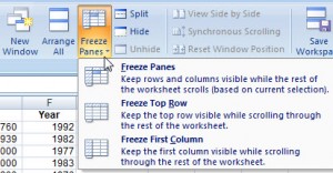
Freeze Panes allows you to “freeze” the row/column labels (for example, “Jan, Feb, Mar, Total”) in view so they continue to show on screen even as you scroll down through document.  Freeze Panes does not affect printing (we’ll cover print-related issues later).

Where you click before you “freeze” is important. Excel will freeze above and to the left of where your cell selection is.  For example, if all you need to freeze is your top row of labels on row 1, click on cell A2 when you Freeze Panes.  If you also need the A column to stay in view when you scroll to the right in a wide spreadsheet, click on cell B2.

            To turn on Freeze Panes:   View  >  Freeze Panes. Choose rows or columns or both.

            To turn off Freeze Panes:  View  >  Unfreeze Panes

[print_link]

If you would like to figure out what a loan payment will be, use Excel’s PMT function.

=PMT(rate,nper,pv,fv,type)

Rate = Interest rate for the loan. Because the interest rate is per annum, you must divide it by 12.
Nper=Number of payments, expressed in years x 12.
Pv=Present Value, otherwise known as the principal or loan amount
Fv=future value, or a cash balance you want to attain after the last payment is made. If fv is omitted, it is assumed to be 0 (zero), that is, the future value of a loan is 0.
Type = (Optional) When payments are due. (Zero or omitted=end of period, 1 is at beginning of period).

The following is an example of a mortgage loan payment calculation:

The function typed in to cell B7 in this illustration is =PMT(B5/12,B6*12,B4).  B5 is the interest rate, which must be divided by 12 because it is an annual rate. B6 is the loan term, which must be multiplied by 12 for the 12 payments per year. B4 is the loan amount. In this example, there is no need to include Future Value or Type. 

Note:  There is also a PPMT function.  PPMT returns the principal portion of a specific loan payment; where PMT returns the full, fixed payment for a loan.

Everyone makes data entry errors. You need to correct errors quickly so you can move on with completing your work. In Excel, here are some ways to do that.

If the error just occurred:

1. [ESC] key on the keyboard. If you are still typing and have not hit [Enter] yet, press [ESC]. This cancels what you’ve begun to type in to a cell, but have not confirmed yet. (If you have already hit [Enter], see instructions below).
2. Click the Red X on the formula bar. This is the same thing as pressing [ESC]. The red X will not be available if you have already entered the data. This is only if you are still typing in the cell.
3. UNDO: If your error is recent, you can Undo. To undo:
Keyboard method – CTRL Z; (This one works in almost all programs)
Toolbar method – Undo Button (Left-facing blue arrow)
Menu method = EDIT > UNDO

If the error has already been entered, you have 2 options:

1. Click on the cell and simply re-type the correct entry. You do not have to press delete first, though that would work as well. The correction can be re-typed in the cell or on the formula bar.
2. Delete: Highlight the cells to delete data from, press [DELETE] on your keyboard.

Remember – UNDO is your best friend!

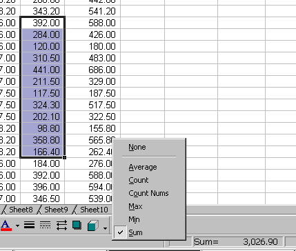
Need a quick total or count without having to write a formula?  Excel’s AutoCalculate will show you a total, a count, an average, or other calculations by simply selecting the cells you are calculating.  Look on the lower right hand portion of the status bar to see the calculated result.

Sum is the default calculation.  To change the type of calculation, right-click on the status bar and choose from the pop-up menu which calculation you want to perform.

Charts are a great way to visually represent and compare data. In
Excel, the key ingredients for a meaningful chart are:

1. Accurate data selected correctly for preparing the chart.
2. The right type of chart for the type of data to be displayed.

QuickTip for an instant column chart

1. Select the comparison data (and labels for the data) to be
   charted.  Example: Sales figures for Jan through June
2. Press [F11] at the top of your keyboard.

If you selected the correct data, you should now have a column chart!

The number one thing you can do to increase your personal
productivity is to get training – and then practice what you learn!